Figure 2.1 Water Flow
This chapter discusses important aspects of a system in general terms.
2.1 Systems in General
A system is a collection of components, interacting for a purpose.
The key words in this definition -- general enough to cover many problems -- are "components" and "interacting". Yet a pair of pliers has components that interact, and is therefore a system, but not one to attract our current attention. The definition is too broad to be useful. It is better to discuss the characteristics of a typical system that might be studied in management science, especially that end of the science concerned with policy analysis.
Systems of interest have something flowing through them, and the flows accumulate in various parts of the system. The flows of a fuel distribution system occur within pipelines, and the flows are accumulated in fuel tanks. An inventory system, an influenza epidemic, and an irrigation system, all have analogous flows and accumulations. A pair of pliers does not.
The "flows" are typically flows of materials that accumulate as "stocks" -- the flows of goods ordered and goods sold, for example, accumulate as a stock held in a warehouse. Material flows should be interpreted in the broadest generic sense. "Material" may be people, or energy, or temperature, or other abstract concepts that can be accumulated. Changes to temperature, for example, may be accumulated as current temperature. Price levels are accumulations of price changes. Modeling will require considerable imagination on what are and are not likely candidates to be material flows in any particular system.
A system encompasses three major concepts. The first is time, the second accumulation, and the third feedback.
Consider a simple inventory system. The inventory changes over time. The change is due to the accumulation of orders. And the order rate changes due to the feedback effect of inventories exceeding or falling short of desired inventory levels.
As time, accumulation, and feedback are so basic to systems, they warrant further discussion.
2.2 The "Time" Variable
By analyzing a system, we mean showing how the system changes over time. This can be done in two ways. First by finding an analytic function that includes all the system variables in a mathematical expression that is a function of time, and then inserting any selected value of time to obtain system values at that point. This analytic approach is virtually impossible in any realistic managerial or social system. There are too many interacting variables to allow solution.
The second method is to simulate the system. This means providing a set of equations that defines each variable in the system as a function of other variables which affect it. Then, given a set of initial conditions -- values for appropriate variables at the start of the simulation -- the system is "simulated" by calculating new values for each variable at each successive time step. Time is the indexing variable. The system variables are calculated as time changes, and the values of the variables are indexed, or subscripted, by the point in time at which they are calculated.
The second method is usually feasible for use in managerial and social systems.
A very important characteristic of time is that it is a truly independent variable (relativity theory aside). It makes sense to make the level of an inventory be a function of time, but it hardly seems practical to make time a function of inventory level. Being an independent (or exogenous) variable, time is an excellent indexing variable. Systems with feedback can be made dependent on time, without concern that time is dependent on the system variables.
There are modeling techniques that use other indexing variables. An "event-based" simulation of an inventory, for example, may define its variables as functions of sales, so that a calculation occurs each time an item is sold. Such indexing is not very suitable however, for most feedback models.
2.3 The Process of Accumulation
A dynamic system is one in which there are flows that, as time passes, are accumulated (or "integrated") into stocks. Flows are often called "rates", for "rate of change" per unit time, of the stock, and stocks are called "levels", representing the amount of flows that have accumulated. The terms "stocks and flows" and "levels and rates" are closely related. A level represents the value for a stock at a point in time, and a rate represents the value for a flow.
Whenever flows -- which can be inflows or outflows are being accumulated or integrated into a level, then the system controlling the process is a dynamic system. That system is in a dynamic state if one or more of the levels in the system are changing, that is the net accumulation rates are not all permanently zero in all the levels. If the net accumulation rates are stable at zero in all levels, the system is in a static state.
For example, consider an irrigation system consisting of two dams placed along a river basin to accumulate two reservoirs (or stocks) of water. During any period of time, each reservoir accumulates the net of its inflow less outflow from its dam. If the reservoir levels of each dam are unchanging, then the outflows equal the inflows and this system is static, there are no net accumulations in any of the dams.
Now assume a thunderstorm occurs in the high country feeding the tributaries above the dam furthest upstream. After a lag, this first reservoir will begin accumulating the rainfall. Its inflow will exceed its outflow and net accumulation for the first dam becomes positive. The system becomes dynamic -- even though the second dam has not yet felt the effect of the rainfall. So long as one level in a system is in a dynamic state, the system -- by definition -- is in a dynamic state. This is also called being in a "transient state".
As the thunderstorm subsides, the first dam will eventually return to a static state, where inflow and outflow are equal, while the second dam absorbs the effects of the storm. Ultimately, the dynamic effects of the storm are gone, as each dam returns to a static condition, and the level of each dam is once again constant.
But note two things. First, the new static levels of each dam may be different than the previous static state. Second, "static" does not necessarily mean there are no accumulations. Each dam can still accumulate inflow, but the inflow now equals the outflow. A static system can have levels, so long as they are unchanging. A system with levels that have stabilized, or become constant, is said to be in "steady state".
There are systems that have no levels (accumulated flows) at all. In the river system just mentioned, the river itself, before the dams were built, could be considered a system without accumulations. Ignoring friction -- and any accumulated water in natural pools along the river -- the purely static river system would simply be a river which flowed either slowly or rapidly, but had no changing stocks or levels.
A more precise version of such a system is a lawn sprinkler system, which has pipes from the water supply to the sprinkler heads. In this system -- static by our definition -- water flows through the pipes, which always contain the same volume and no accumulations.
Often, in "systems analysis" or other forms of management science, a system is analyzed, and results are presented for the system only in its steady state. This allows solution through static analytic methods, mathematically tractable and academically satisfying, but somewhat unrealistic.
To be specific, if an inherently dynamic system is assumed to have reached steady state, then the analysis of the system simply requires making the inflows to each level equal its outflows. Equalizing these flow rates provides an "equilibrium condition" for each level, and the condition is algebraic ... that is, there are no derivatives or integrals involved in the equation. Simultaneously considering the individual equilibrium conditions for each level allows solving a set of simultaneous algebraic equations -- instead of solving the inherent differential equations needed to define the transient state. Said another way, algebra can be used to solve the system equations, instead of calculus. This is convenient mathematically, but avoids exploration of the transient dynamics that accompany most systems.
But policy analysts need no longer emphasize steady state analysis. Modern computers and software have made it feasible to explore dynamic systems. After all, knowing that the nation's unemployment rate will reach four percent in steady state, is not comforting if the rate fluctuates between 12 percent, four, eight, five, and so on, before stabilizing at four percent ... especially since policy and economic changes will no doubt prevent the steady state from ever occurring!
2.4 Feedback Systems
A system can have accumulations -- be dynamic without having feedback. Systems that vary over time without feedbacks have been referred to as being "dynamic in the weak sense", while those having feedback have been called "dynamic in the strong sense" [Brems, 1973]. The difference lies in the concept of feedback.
Feedback, for our purposes, means that at least one variable in a system is affected by another variable, which was earlier affected by the first. In other words, there is a "feedback loop" somewhere in the system.
For example, the rate of new births in a population is affected by the population size, and of course the population size depends on the rate of new births. That is feedback by our definition.
The feedback characteristic is the ingredient that complicates the mathematical solution of a system. The following simple exercise sequence is intended to show the increase in conceptual difficulty that occurs in going from a static system, to a dynamic system, to a dynamic feedback system.
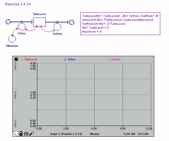
Exercise 2.4.1 A Water Flow Problem
The following three exercises demonstrate, respectively, static, dynamic, and feedback conditions. The problem uses several concepts not yet fully developed. The reader new to systems theory may want to follow the problem logic without becoming overly concerned if, for now, portions of it seem still undefined.
Exercise 2.4.1A: Water flows into a tank at a rate inversely proportional to the level in the tank. The inflow is 1 gallon per minute at time zero when the tank is empty, and 0 when the tank contains four gallons. In other words, the inflow rate can be defined mathematically:
INFLOW(t,t+dt) = 1 * (4-LEVEL(t))/4,where * is the symbol for multiplication, dt is a small increment of time, INFLOW(t,t+dt) is the value of the inflow between time t and t+dt, and where LEVEL(t) is the value of the variable LEVEL at time t.
Further, an outflow valve lets water flow out of the tank at a rate equal to 0.2 times the number of gallons in the tank. What is the steady state level of water in the tank, and what does the flow equal at steady state, that is, when the inflow equals the outflow and the level of water in the tank has stabilized? The answers are provided at the end of this section.
Exercise 2.4.1B: Water flows into a tank with no outflow. At time zero, the tank is empty and the inflow is 1 gallon per minute. The inflow decreases proportionally each minute with time until time 4, when the flow is zero. In other words, the inflow rate is
INFLOW(t,t+dt)) = 1 * (4-TIME(t))/4,and the level at time t=T is
LEVEL(T) = SUM(INFLOW(t-dt,t); t=dt,T),where SUM(INFLOW(t-dt,t); t=dt,T) means
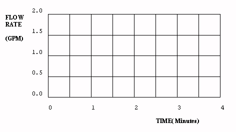
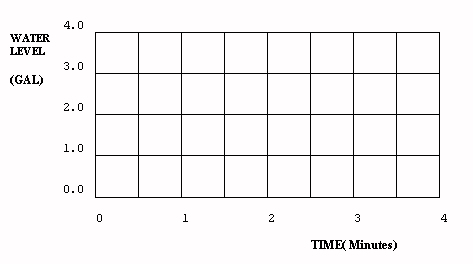
INFLOW(0,dt) + INFLOW(dt,2dt) + ... + INFLOW(T-dt,T).What are the values for the level and the rate of flow of water into the tank over time? Use the following graphs to obtain an approximate solution (or solve the problem mathematically using calculus). To simplify the analysis, assume dt=1 in the above equations.
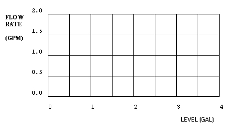
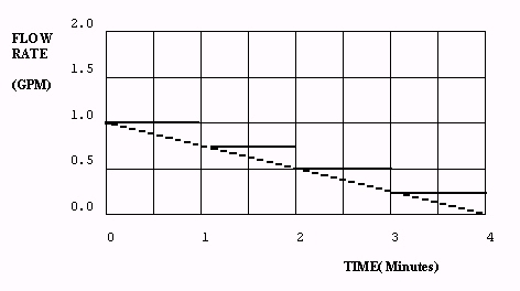
Exercise 2.4.1C: Water flows into a tank with no outflow. The inflow is 1 gallon per minute when the tank is empty, and decreases proportionately with the water level until the level equals 4 gallons, when the flow is zero. In other words, the inflow rate is
Answers to 2.4.1: Water Flow Problem
Answer 2.4.1A: At steady state, the water inflow equals the outflow. Assume the symbol ¥ means "a very large number" and let any variable FLOW(¥ ,¥ +1) be designated FLOW(¥ ). Then mathematically,
INFLOW(¥ ) = 1 * (4-LEVEL(¥ ))/4 (2.4.1)and INFLOW = OUTFLOW, the equilibrium condition, impliesOUTFLOW(¥ ) = .2 * (LEVEL(¥ )) (2.4.2)
LEVEL(¥ ) = 2.22 GALLONS, andThese are the steady state values obtained by solving the equilibrium condition using equations 2.4.1 and 2.4.2. This is a static mathematical exercise, as there are no difference equations.INFLOW(¥ ) = OUTFLOW(¥ ) = .444 gallons/min.
Answer 2.4.1B: This problem has accumulation, but no feedback, the variable INFLOW is dependent on time, and time is always independent, therefore exogenous to the problem. The graphical solution is thus easily derived, and is shown. The system is "iterated" through time by starting with the initial conditions (water level equals zero at time zero), then adding to the level, each one minute time step (dt=1), the amount of water that has flowed into the level since the last iteration. The solid lines of Figure 2.4 show the results of this iterative process.
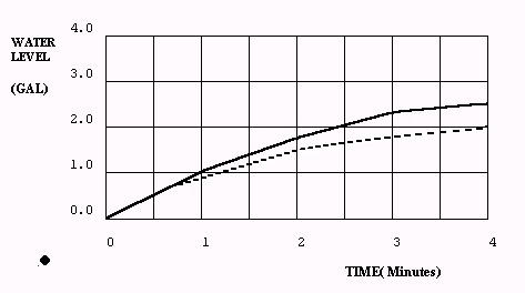
Iteration, and the treatment of time and time intervals, will be discussed more fully in section 3.4. For now, note that iterating the solutions at one minute intervals causes inaccuracies. The solid lines in the figure show how flow rates are held constant for a entire time step. The dashed lines show the correct flows and levels, when flows change continuously instead of in discrete time steps. The dashed line solution results from the calculus solution provided at the end of this exercise. Accuracy increases if dt is reduced, but the number of calculations expands. Note also that the level, being an accumulation, has a value equal to the area under the flow graphed to that point.
Answer 2.4.1C: When the inflow rate depends on the level, instead of on the exogenous variable time, the system has feedback as well as accumulation. Feedback complicates the solution significantly, as the inflow rate affects the water level, and the water level affects the inflow rate. A graphical solution requires first finding the flow rate at each time step, then calculating the level, recalculating the flow for the next time step, then recalculating the level, and so forth.
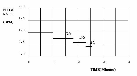
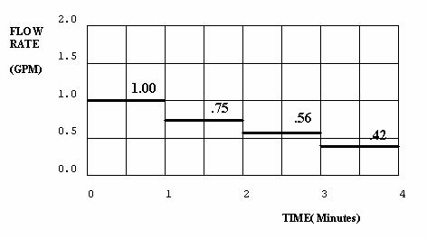
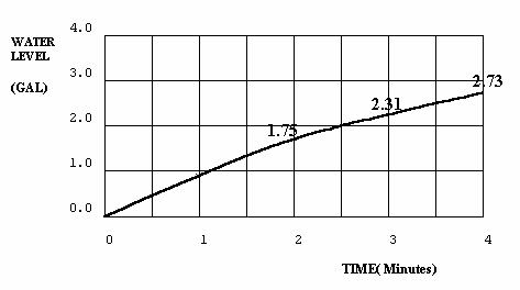
Figure 2.6 - Plots of Variables Exercise 2.4.1C
Digression: Mathematical solutions to exercises 2.4.1B and 2.4.1C provide insight. Using calculus, the rate of flow in exercise B can be written as the change in level with respect to time (the "derivative").
dL/dt = 1 * (4-t)/4; 0<t<4. (2.4.3)Note that dL/dt is only a function of t. The solution to 2.4.3 is (separating variables and using direct integration to solve the differential equation)
L(t) = t t**2 /8, (2.4.4)Where ** means "raised to the power of".
In exercise C, the rate of flow is
dL/dt = (4-L(t))/4; 0<L<4. (2.4.5)Here dL/dt is a function of both L and t, and the problem is more sophisticated. Solving 2.4.5, a very simple linear differential equation, is already nontrivial. The solution method, found in any basic calculus text, leads to
L(t) = 4 - 4e**(-t/4) (2.4.6)2.4.4 and 2.4.6 can be checked by the reader to confirm they fit the conditions of the exercise, for example, when t=0, L=0.
Exercise 2.4.1 has represented a very simple system. The mathematical digression was meant to show how analytically solving a system rapidly becomes difficult as the number of levels in a system increases and the interactions of their rates of flow becomes more complex. Systems with over three or four levels become difficult, mathematically. A social system with 10 or 15 levels simply cannot be solved analytically.
2.5 Conservative Flows and Informational Flows
We have discussed two systems components -- levels and rates (or stocks and flows). Any particle of material being processed in a system can only be in one place at any point in time, and it must either be in a rate flowing between two levels, or be in a level.
Rates and levels, therefore, are considered to encompass the "conservative" parts of a system. Material flowing from a source is no longer at that source; material transferred from one part of the system to another cannot be in both places; material cannot be transferred to more than one place at a time. This is not so with information.
Information about material in one part of the system can be tranferred to several other parts, yet the material still remains at the source. Information flow is not conservative. Information on the level of inventory held at the end of the month, for example, could be used by the marketing department to affect the advertising rate. It could also be used by sales to affect the rate of price changes, and by purchasing to affect the ordering rate. Information taken from a source remains at the source.
In all systems, the rates of flow control the system, and the values of the rates depend on information about the system's levels. This may be clearer if rates are compared with levels. A level changes as, and only as, material flows into or out of the level ... the level depends on rates directly connected to it. Rates depend on levels, but not in an analogous way. A rate can depend on a level not connected to the rate. The rate of population deaths, for example, can be a direct function of air polution, a level defined in a completely different part of the system. However the polution level could not be directly affected by population deaths.
A key difference, then, is that levels depend on material flows connected to them, while rates depend on information links to levels anywhere in the system. These information links to levels are functional relationships that can become quite complex mathematically, and therefore are often decomposed through the use of intermediate variables, called "auxiliaries". Auxiliaries can be functions of levels, rates, or other auxiliaries. These functions help clarify the definition of rates and their ultimate dependence on the system levels.
The relationship between levels, rates, and auxiliaries, will become clear when they are diagrammed in sections 4.2 and 4.3, but as an example, consider the inventory level for a microcomputer store. Computers are ordered and accumulate in the store's inventory, and are sold. The desired inventory level (a constant) is 100 computers. In this system, the rate of arrival of computers is a flow, the rate of sales is a flow, the accumulated computers in the inventory is a stock, and the information variable "desired inventory minus actual inventory" is an auxiliary that controls orders for new computers. If, over time, average weekly sales of computers (which depends on weekly sales) rises permanently, then the desired inventory level may change to a new value. Desired inventory, if dependent on average sales, ceases being a constant, and becomes another information auxiliary.
The control variable in this problem is the flow of orders placed with the manufacturer, which affects the flow of computers arriving at the store.
Control variables are the rates used by management to control systems. Proper control of the control variables will cause the system to respond properly, while poor control will cause undesired system responses. Managerial control invariably depends on information about the system's status. Consequently control variables respond to information -- information which depends on the status of the system's levels, which, after a time lag, depend on the control variables. That is the feedback nature of systems.
2.6 Variables, Parameters, and System Boundaries
Rates, levels, and auxiliaries have all been called variables. Each of these system components indeed vary as the system changes. These system variables are more correctly called "endogenous variables", as they are determined internal to the system.
Variables that do not depend on other system variables can be refered to as "exogenous variables", as their values are determined outside the system. Time is the most common exogenous variable -- its value changes, but is not dependent on the values of system variables.
The opposite term to "variable" is "parameter". Constants are parameters. In an inventory problem, the delivery delay between placing an order from the manufacturer and receiving the order in inventory may be a constant, say three days. The delivery delay is a parameter.
The sales rate, on the other hand, may vary only with time of year (being high in the summer and low in the winter), or vary randomly from week to week. In this example, sales rate is an exogenous variable -- it does not depend on other endogenous system variables.
Inventory level, however, depends on deliveries, which is a system variable depending on inventory. Inventory level is an endogenous variable, as, by the way, is the delivery rate. When we refer to system variables, we shall mean endogenous variables.
The key difference between system variables and either parameters or exogenous variables, is that system variables depend on other variables within the system, while parameters and exogenous variables depend on things outside the system. Parameters and exogenous variables are typically determined through statistical methods such as estimation, regression, and forecasting. Parameters and exogenous variables then, are the links that connect the variables within a system to the environment outside the system; they cross the system boundary.
2.7 The System Boundary
When studying a system and how the system changes, the modeler must identify the variables of major interest. The boundary of the system being modeled should circumscribe all such variables. System variables are related to exogenous variables and parameters external to the model either through the use of analytic functions, or through "table functions" which are described later.
The boundary is often not explicitly defined in the modeling process.
It implicitly contains all variables that are defined as dependent on other
variables, and excludes those only dependent on constants or exogenous
variables. In figure 2.7.1, recruitment, labor supply, resignation, and
labor demand are endogenous variables. Recruitment and resignation depend
on (exogenous) pay scales and unemployment rates, and labor demand depends
on the
(exogenous) military threat.
In figure 2.7.2, the modeler has made pay scales endogenous, feeling that if military labor supply and demand are mismatched, the organization under study can affect pay scales to help correct the mismatch.
These figures introduce influence diagrams typical in model building. The arrows show the direction of causal influence. For example, the larger the labor supply, the larger the resignation rate, and the larger the resignation rate the less the labor supply.
In most model efforts there will be certain variables that are neither clearly endogenous or exogenous. In a military manpower planning process, for example, recruiting rates are dependent on advertising budgets and military pay rates, and all three are likely to be endogenous variables. Recruiting rates are also dependent on the demographics of the nation's l8-21 year olds, and the size of this labor pool can be provided to the model as a time dependent exogenous variable. However, while the pool of all 18-21 year olds is virtually independent of the military recruiting rate, the 18-21 year olds willing to join the military may be dependent on the economic health of the nation's private sector, which in turn may depend partly on military expenditures. It then becomes difficult to decide whether to make the available 18-21 year old population an exogenous variable to be provided when needed by the model, or expand the model to include the economy as a whole and split the 18-21 year old population into two endogenous variables -- one of those willing to join and the other of those unwilling, with the ratio dependent on economic health. In this example, the model expansion would be so major that the modeler would probably choose to make the labor pool variable exogenous, and provide a table for the labor pool as a function of time.
One of the modeler's most difficult tasks is the determination of the system boundary. Usually one starts with the variables known to be internal, and then forms linkages until potential system boundaries are reached. Often the final boundary is not determined until late in the model building stage. The compromises made in determining which variables to include and which to exclude will often be less than obvious. Some arbitrary decisions will need to be made. Incidently, these decisions should be documented, as model justification will be facilitated later if a time track of model decisions is recorded.
2.8 Model Sectors
The model boundary contains endogenous variables linked to the environment through parameters and exogenous variables. It isolates the system under study. Within the boundary, most models contain subsystems or "sectors" linked to variables in other sectors. These linkages are similar to those linking the model variables to the environment, but in this case the linkage is through system variables. Variables in a sector will change as the variables to which they are linked change.
For example, in a small supplier's inventory problem, one sector might be the inventory sector, comprised of the inventory, orders, average sales, and desired inventory. Sales and delivery delay are exogenous. Orders and sales affect inventory, desired inventory depends on average sales, and orders depend on the difference between desired inventory and inventory. Figure 2.8.1 applies.
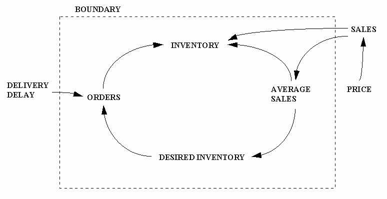
Figure 2.8.2 Sales and Inventory Model
Sales would be inversely related to price, another new endogenous variable. Sales and price now form a pricing sector, price being affected by the imbalance between desired and actual inventories.
This example may clarify the difference between endogenous system variables,
and exogenous variables. With sales an exogenous variable, sales will vary
with time, but the sales profile over time will be identical, no matter
how the system is controlled. On the other hand, if sales depend on price,
and price is endogenous, then the sales profile over time will be
different for different ordering and pricing policies.
Clearly the latter problem is more complex, and difficult to solve analytically.
Yet it is easy to analyze using a stock/flow approach. This highlights
why system dynamics is an appropriate method for use by the management
scientist.
(c) 1999 Rolf Clark and John H. Saunders